The Data-Centric Graph Tech Stack

The Data-Centric Graph Tech Stack 

Virtually all technology projects these days start with a “tech stack.” The tech stack is a primarily a description of the languages, libraries and middleware that will be  used to implement a project. Data-Centric projects too, have a stack, but the relative importance of some parts of the stack are different in data-centric than traditional applications.  

This article started life as the appendix to the book “Real Time Financial Accounting,  the Data-Centric Way” and as a result it may emphasize features of interest to accounting a bit more, than otherwise, but hopefully will still be helpful.  

Typical Tech Stacks 

Here is a classic example of a tech stack, or really this is more of a Chinese menu to  select your tech stack from (I don’t think most architects would pick all of these) 

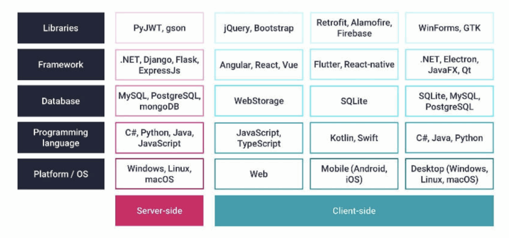
A traditional Tech Stack 

Most of defining a stack is choosing among these. The choices will influence the  capabilities of the final product, and they will especially define what will be easy and  what will be hard. There are also dependencies in the stack. It used to be that the hardware (platform / OS) was the first and most important choice to make and the others were options on top of that. For instance, if you picked the DEC VAX as your platform you had a limited number of databases and even a limited number of languages to choose from.

But these days many of the constraining choices have been abstracted away. When  you select a cloud-based database, you might not even know what the operating  system or database is. And the ubiquity of browser based front ends has abstracted away a lot of the differences there as well.  

But that doesn’t mean there aren’t tradeoffs and constraints. One of the tradeoffs is longevity. If you pick a trendy stack, it may not have the same half-life as one that  has been around a long while (although you might get lucky). And your choice of stack may influence the kind of developers you can attract.  

Every decade or so there seem to be new camps that develop. For a while it was java stacks v C# and .Net stacks. Now a days two of the mainstream camps are react/ JavaScript v. python. Yes, there are many more but those two seem to get a lot of attention.  

React/JavaScript seems to be the choice when UI development is the dominant activity and python when data wrangling, NLP and AI are top of mind.  

Data-Centric Graph Stack 

For those of us pursuing data-centric, the languages are important, but less so than with traditional development. A traditional development project with hundreds of  interactive use cases is going to be concerned with tools that will help with the  productivity and quality of the user experience.  

In a mostly model-driven (we’ll get to that in a minute) data-centric environment,  we’re trying to drastically reduce (close to zero) the amount of custom code that is written per each use case. In the extreme case, if there is no user interface code, it doesn’t really matter what language it wasn’t written it.  

And on the other side if your data wrangling will involve hundreds of pipelines the ease at which each step is defined and combined will be a big factor. But when we focus on data at rest, rather than data flow, the tradeoffs change again.  

Model Driven Development (short version)

In a traditional application user interface, the presentation and especially the behavior of the user interface is written in software code. If you have 100 user interfaces you will have 100 programs, typically each of them many thousand lines of code that access the data from a database, move it around in the DOM (the in memory data model of a web based app as an example) present it in the many fields in the user interface, manage the validation and constraint management and posting back to the database.

In a model driven environment rather than coding each user interface, you code one prototypical user interface and then adapt it parametrically. In a traditional environment you might have one form that has person, social security number and tax status and another form that has project name, sponsor, project management,  start date and budget. Each would be a separate program. The model driven approach says we have one program, and you just send it a list of fields. The first example would get three fields and the second five. It’s obviously not that simple,  and there are limits to what you can do this way, but we’ve found for many enterprise applications you can get good functionality for 90+% of your use cases  this way.  

If you only write one program, and the hundreds of use cases are “just parameters”  (we’ll get back to them later) that’s why we say it doesn’t matter what language you don’t write your programs in.  

One more quick thought on model driven (which by the way Gartner tends to call  low code / no code) is there are two approaches. One approach is code generation.  In that approach you write one program that writes the hundreds of application programs for you. This is likely what we’ll see from GenAI in the very near future, if not already. Some practitioners go into the generated code and tweak it to get exactly what they want. In that case it matters a great deal what language its written in.  

But the other approach does not generate any code. The one bit of architectural  code treats the definition of the form as if it were data and does what is  appropriate.  

Back to the Graph Stack 

So, if we not overly focused on the programming languages what are we focused  on, and why? In order for this discussion to make sense, we need to lay out a few concepts and distinctions, so that the priorities can make sense.  

One of the big changes is the reliance on graph structures. We need to get on the  same page about this before we proceed, which will require a bit of backtracking as  to what the predominant alternatives are and how they differ.  

Proto truths 

We’re going to employ a pedagogical approach using “proto-truths.” Much of the technology we’re about to describe has deep and often arcane specifics.  Technologists feel the need to drill down and explain all the variations of every new concept they introduce, which often gets in the way of the readers grasping the gestalt, such that they could, in due course appreciate the specifics.  

The proto-truth approach says when we introduce a new concept, we’re going to describe it in a simplified way. This simplified way takes a subset of the concept,  often the most exemplar subset, and describes the concept and how it fits with  other concepts using the exemplars. Once we’ve conveyed how all the pieces fit  together, we will cycle back and explain how the concepts work with less exemplar  definitions. For technical readers we will mention that it is a proto-truth every time  we introduce one, lest you say in your mind “no that isn’t the full definition of that  concept.”

Structured Data 

A graph is a different way of representing structured information. Two more  common ways are tables and “documents.” Documents is in quotes here, as depending on your background you may read that and think Microsoft Word, or you may think json. Here we will mean the latter. But first let’s talk about tables as an organizing principle for structured data.  

Tables 

We use tables in relational databases as well as in spreadsheets, and we cut and  paste them into financial reports.  

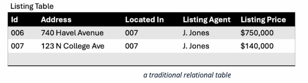
In a table the data is in the cell. The meaning of the data is contextual. This context includes the row and column, but it also includes the database and the table. One allure of tables is their simplicity. But the downside is there is a lot of context for a human to know, especially when you consider that a large firm will have millions of tables. Most firms are currently trying to get a handle on their data explosion,  including processes to document (sorry – different form of the word document)  what all the databases, tables and columns mean. Collectively, these are the  structured data’s “meta-data.” This is hard work, and most firms can only get a partial view, but even partial is quite helpful.   

In “table-world” even if you know what all the databases, tables and columns mean,  you are only part way home. As a famous writer once said: 

“There is a lot more to being a good writer than knowing a lot of good words. You … have … to … put … them … in … the … right … order.”  

In an analogous way to writers putting words in the right order, people who deal  with tabular data spend much of their time reassembling tables into something  useful. It is rare that all the information you needed is in a single table. If it is, it is  likely that one of your predecessors assembled it from other tables and so  happened to do so in a way that benefits you.  

This process of assembling tables from other tables is called “joining.” It sounds simple in classroom descriptions. You “merely” declare the column of one table that is to be joined (via matching) to another table.  

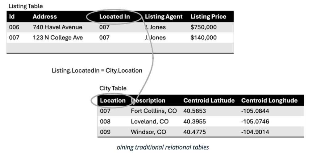
But think about this for a few minutes. The person “joining” the tables needs to  have considerable external knowledge about which columns would be good  candidates to join to which others. Most combinations make no sense at all and will get little or no result. You could join the zip code on a table of addresses with the salaries of physicians, but the only matches you’d get would be a few underpaid physicians on the West coast. 

This only scratches the surface of the problem with tables. This “joining” approach only works for tables in the same database. Most tables are not in the same database. Large firms have thousands of databases. To solve this problem, people  “extract” tables from several databases and send them somewhere else where they can be joined. This partially explains the incredible explosion of numbers of tables that can be found in most enterprises.  

The big problem with table based systems is how rapidly the number of tables can explode, and as it does the difficulty of know which table to access, what the  columns mean and how to join them back together becomes a bit barrier to productivity. In a relational database the meaning of the columns (if defined at all)  is not in the table. It might be in something the database vendor calls a “directory”  but more likely its in another application, a “data dictionary” or a “data catalog.” 

This was a bit of a torturous explanation of just a small aspect of how traditional  databases work. We did this to motivate the explanation of the alternative. We know from decades of explaining; the new technology sounds complex. If you really  understand how difficult the status quo is, you are ready to appreciate something  better. And by the way we should all appreciate the many people who toil behind the scenes to keep the existing systems functioning. It is yeoman’s work and should be applauded. At the same time, we can entertain a future that requires far less of this yeoman’s work.

Documents 

Documents, in this sense, as a store of structured information, are not the same as  “unstructured documents.” Unstructured documents are narrative, written and read by humans. Microsoft Word, PDFs and emails are mostly unstructured. They may have a bit of structured information cut and pasted in, and they often have a bit of “meta-data” associated with them. This meta-data is different than the meta-data in tables. In tables the meta-data is primarily about the tables and columns  and what they mean. For an unstructured document, meta-data is typically the author, maybe the format, the date created and last modified date, and often some tags supplied by the author to help others search later.  

Documents in the Document Database sense though are a bit different. The exemplars here are XML and json (JavaScript Object Notation).  

XML JSON 

semi structured “documents” 

The difference here between tables and documents is that with documents the  equivalent of their meta-data (part of it anyway) is co-located with the data itself.  The json version is a bit more compact and easier to read, so we’ll use json for the rest of this section.  

The key (if you pardon the pun) to understanding json lies in understanding the key/value concept. The json equivalent to a column in a table is the key. The json equivalent to a cell in a table is a value. In the above, “city” is a key, and “Fort  Collins” is a value. Everything surrounding the key/value pair is structure or context.  For instance, you can group all the key/value pairs that would have made up a row in a table, inside a matching pair of “{ }”s. The nesting that you see so often in json (where you have “{… }” inside another “{ …}” or “[…]” ) is mostly the equivalent of a join.  

An individual file, with a collection of json in it, is often called a dataset. A dataset is a mostly self-contained data structure that serves some specific purpose. These  files / datasets look and act like documents. They are documents, just not the type for casual reading. When people put a lot of them in a database for easier querying,  this is called a “document database.” They are handy and powerful, but unless you know what the keys and the structure mean, you don’t know what the data means.  The number and complexity of these datasets can be overwhelming. Again, kudos  to the many men and women who manage these and keep everything running, but again, we can do better.  

Graph view of tables or documents 

Many readers already familiar with graph technology will be raising their hands  right now and saying things like “what about R2RML or json-LD?” Yes, there are  ways to make tables and documents look like graphs, and consume like graphs, but  this never occurs to the people using tables and documents. This occurs to the people using graph who want to consume this legacy data. And we will get to this,  but first we need to deal with graphs and what makes them different (and better). 

Graph as a Structuring Mechanism 

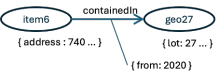
In graph technology, the primitive (and only) way of representing information is in a  “triple.” A triple has three parts: two nodes and an edge connecting them.  

graph fundamentals 

At the proto-truth level, the nodes represent individual real-world instances,  sometimes called individuals. In this context individual is not a synonym for person,  for instance in this example we have an individual house on an individual lot.  

things not strings 

These parenthetic comments are just for the reader, in a few moments we’ll fill in how we know the node on the left represents a particular house and the node on  the right an individual lot that the house is on.

The line between the individuals indicates that there is some sort of relationship between the individuals.  

naming the edges 

In this case, the relationship indicates that the house is located at (on) the specific lot. The lot is not located at or on the house, and so we introduce the idea of directionality.  

edges are directional 

The node/edge/node is the basic graph structure and that the edge is “directed”  that is, has an arrow on the end, makes this a “directed graph.” 

There are two major types of graph databases in current use: labeled property graphs and RDF Databases, which are also known as Triple Stores. Labeled property graphs, such as the very popular Neo4j, are essentially document stores with graph features. The above triple might look more like this in a labeled property graph: 

Attributes on the edges 

Each node has a small document with all the known attributes for that node, in this case we’re showing the address, and the lot for the two nodes. The edge also has a small document hanging off it. This is what some people call “attributes on the edges” and can be a very handy feature. Astute readers will notice that we left the  “:” off the front of the node and edge names in this picture. We will fill in that detail in a bit.  

Triple stores do not yet have this feature (attributes on the edges) universally implemented, it is working its way through the standards committees, but there are  still several reasons to consider RDF Triple stores. If you choose not to implement an RDF Triple store for your Data-Centric system, these Labeled Property Graphs are probably your next best bet. Both types of graph databases are going to be far easier than relational or document databases for solving the many issues that will  need to be dealt with going forward.  

Triple stores have these additional features which we think make them especially  suitable for building out this type of system: 

• They are W3C open standards compatible – there are a dozen viable commercial options and many good open-source options available. They are very compatible. Converting from one triple store to another or combining two in production is very straightforward.  

• They support unambiguous identifiers – all nodes and all edges are defined by globally unique and potentially resolvable identifiers (more later) • They support the definition of unambiguous meaning (semantics) – also more later.  

We have a few proto-truths that we have skipped over that we can fill in before we  proceed. They have to do with “where did these things that look like identifiers  come from and what do they signify?” 

Figure 1 — the basic “triple” 

The leading “:” is a presentation shorthand for a much longer identifier. In most  cases there is a specific shorthand for this contextualizing information, which is  called a “namespace.” The namespace represents a coherent vocabulary, and any triplestore can mix and match information from multiple vocabularies/  namespaces.  

Figure 2 — introducing namespaces   

In this example we show these items coming from three different namespaces or vocabularies. The one on the left: “rel:” might be short for a realtor group that  identified the house. The “gist:” refers to an open-source ontology provided by  Semantic Arts and the “geoN:” is short for geoNames – another open-source vocabulary of geospatial information. The examples without any qualifiers (the ones with only “:”) still have a namespace but it is whatever the local environment has declared to be the default. 

Let’s inflate the identifier:  

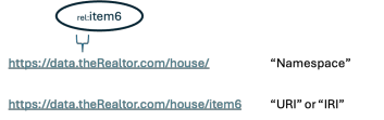
Prefixes are Shorthand for Namespaces  

The “rel:”is just a local prefix that will get expanded anytime this data is to be stored  or compared. The local environment fills in the full name of the namespace as shown here (a hypothetical example). The namespace is concatenated with what is  called the “fragment” (the “item6” in this example) to get the real identifier, the “URI”  or “IRI.”

IRIs are globally unique. So are “guids” (Globally Unique IDentifiers). 

guids as globally unique ids 

Being globally unique has some incredible advantages that we will get to in a  minute, but before we do, we want to spend a minute to distinguish guids from  IRIs. This guid (which I just generated a few minutes ago) may indeed be globally unique, but I have no idea where to go to find out what it represents.  

The namespace portion of the IRI gives us a route to meaning and identity. 

Using Domain Names in Namespaces to Achieve Global Uniqueness  

Best practice (followed by 99% of all triple store implementations) is to base the  namespace on a domain name that you own or have control over. As the owner of the domain name, and by extension the name space, you have the exclusive right to “mint” IRIs in this namespace. “Minting” is the process of making up new IRIs.  With that right comes the responsibility to not reuse the same IRI for two different things. This is how global uniqueness is maintained in Triple Stores. It also provides  the mechanism to find out what something means. If you want to know what  https://data.theRealtor.com/house/item6 refers to you can at least ask the owners of theRealtor.com. In many cases the domain name owner will go one step further,  and not only guarantee that the identifier is globally unique, but they will tell you  what it means in a process call “resolution.” An IRI, following this convention, looks a lot like a URL. The minter of this IRI can, and often does, make the IRI resolvable.  To the general public the resolution may just say that it is a house and here is its  address. If you are logged in and authenticated it may tell you a lot more, such as who the listing agent is and what the current asking price is.  

The URI/IRI provides an identifier that is both resolvable and globally unique.  Resolvable means you have the potential of finding out what an identifier refers to.  Let’s return to the value of global identifiers.  

In the tabular, document and even labeled property graph, the identifiers are  hyper-local. That is an identifier such as “007” only means what you think it means  in a given database, table and column.  

Figure 3 — Traditional systems require the query-er to reassemble tables into small graphs to get anything done 

That same “007” could refer to a secret agent in the secret agent database, and a ham sandwich in the deli database. More importantly, if we want to know who has  the Aston Martin this week we need to know, as humans, that we “join” the “id” column in the “agent table” with the “assigned to” column in the “car” table. This doesn’t scale and it’s completely unnecessary.  

When you have global ids, you don’t need to refer to any meta data to assemble data. The system does it all for you. https://data.hmss.org.uk/agent/007 refers to  James Bond no matter what table or column you find it in or if you find it on a web site or in a document.  

Say we found or harvested these factoids and converted them to “triples”. This is depicted in the figure below. For readability, we’ve temporarily dropped the namespace prefixes and added in parenthetical comments. 

Triples sourced independently 

The first triple says the house is on a particular lot. The second triple says what city that lot is in. The third adds that it is also in a flood plain. The fourth, which we  might have gotten from county records, says there is a utility easement on this lot.  And the last is an inspection that was about this house (note the arrow pointing in  the other direction). 

The database takes all the IRIs that are identical and joins them. This is what people normally think of when they think of a graph. 

Triples Auto-snapped Together

  

Notice that no metadata, was involved in assembling this data into a useful set and note that no human wrote any joins. Hopefully this hints at the potential. Any data we find from any source can be united, flexibly. If a different lot had 100 facts about it, that would be ok. We are not bound by some rigid structure.  

Triples 

But we still have a few more distinctions we’ve introduced without elaborating.  

We introduced the “triple,” but didn’t elaborate. A triple is an assertion, like a small  statement or sentence. It has the form: subject, predicate, object. In this case:
  :item6 (subject), :hasPhysicalLocation (predicate), :geo27 (object).  

(subject) (predicate) (object) 

Triples as Tiny Sentences 

The one we showed backward should be read from the tail to the head of the arrow.  

Read Triples in the Direction of the Arrow 

The :insp44 (subject) :isAbout (predicate) :item6 (object).  

A Schema Emerging 

You may be willing to accept that behind the scenes we did something called “Entity  Resolution.” This is very similar to what it is in traditional systems; it is the gathering up of clues about an entity (in this case the house, the lot, the city etc.) to determine whether the new fact is about the same entity we already have information about.  

Assuming we have the software, and we are competent, we can figure out from  clues (which we’ve skipped over so far) to determine that all facts about item6 are  in fact about the same house. And that also behind the scenes we came up with  some way to assign a unique fragment to the house (in this case the unusually  short, but ok for the illustration “item6.”) 

But you should wonder where did “:hasPhysicalLocation” come from. Truth is, we  didn’t just make it up on the fly. This is the first part of the schema of this graph database. It must have existed before we could make this assertion using it. 

We are going to draw this a bit differently, but trust us, everything is done in triples,  it is just that some triples are a bit more primitive and special and well known than others. In this case we created a bit of terminology before we created that first triple. We declared that there was a “property” that we could reuse later. We did it  something like this: 

Schema are Triples too! 

This is the beginning of an “ontology” which is a semantic data model of a domain.  It is built with triples, exactly as everything else is, but it uses some primitive terms that came with the standards. In this case the RDF standard1 gives us the ability to declare a type for things, and in this case, we use the OWL standard 2to assert that this “property” is an object property. What that means is that it can be used to connect two nodes together, which is what we did in the prior example.  

We’ve noticed that having everything be triples kind of messes with your mind when you first pick this up so we’re going to introduce a drawing convention, but keep in mind this is just a drawing convention to make it easier to understand,  behind the scenes everything is triples, which is a very good thing as we’ll get to later.  

There is something pretty cool going on here. The metadata, and therefore the  meaning, of data is co-located with the data, using the same structural mechanics  as the data itself. This is not what you find in traditional systems. In traditional systems the meta data is typically in a different syntax (DDL Data Definition  Language is the metadata language for relational and DML Data Manipulation  Language is its manipulation language), which is often in a different location (the directory as opposed to the data tables themselves) and is often augmented with more metadata, entirely elsewhere, initially in a data dictionary, and more recently in data catalogs, metadata management systems and enterprise glossary systems.  With Graph Databases once you get used to the idea that the metadata is always right there, one triple away, you wonder how we lived so long without it.  

In our drawing convention, this boxy arrow (which we call “defining a property”):

Shorthand for Defining a Property 

Is shorthand for this declaration: 

Defining a Property as Triples 

Which makes it easier to see, when we want to use this property as a predicate in  an assertion: 

Defining a Property v. Using it as a Predicate in a Triple 

This dotted line means that the predicate refers to the property, there isn’t really another triple there, in fact the two IRIs are the same. The one in the boxy arrow is  defining what the property means. The one on the arrow is using that meaning to make a sensible assertion.  

When we create a new property, we will add additional information to it (narrative to describe what it means, and additional semantic properties, but rather than clutter up the explanation, let’s just accept that there is more than just a label when you create a new property).  

Classes 

You may have noticed that we haven’t introduced any “classes” yet. This was intentional. Most design methodologies start with classes. But classes in traditional technology are very limiting. In relational “class” equals “table.” That is, the class tells you what attributes (columns) you can have, and in so doing limits you to what attributes you can have. If one row wants more attributes you must either grant them for all the rows in the table, or build a new table, for this new type of row.  

In semantics the relationship between individuals and classes is quite different. A  class is a set. We declare membership in a set by, (wait for it) a triple.  

While this is all done with triples, once again they are pretty special triples, that are called out in the standards. In order for us to say that item6 is a House, we first had to create the class House.

Class Definition as Triples 

Again, because we humans like to think of schema or metadata differently than  instance data, we will draw classes differently — but keep in mind this is just a  drawing convention and is a bit more economical on ink. 

A shorthand for asserting an instance to be a member of a class 

The incredible power comes when you free yourself from the idea that an instance  (a row in a relational database) can only be in one class (table). When relational people want to say that something is a both a X (House) and a Y (Duplex) the copy the id into a different table, and export the complexity to the consumer of the data to know that they have to reassemble it.. 

Instances can be members of more than one class 

In Object Oriented design, we might say that a Duplex is a sub type of a House. (all duplexes are houses not all houses are duplexes), but this is at the class level,  which ends up being surprisingly limiting.  

Now there might be a relationship between Duplex and House, but what if we also  said 

The classes themselves need not have any pre-existing relationship to each other 

Maybe because you’re an insurance company or a fire department and you’re interested in which homes are made of brick. Note that many brick buildings are  neither houses nor duplexes (they can be hospitals, warehouses or outhouses). In  any event this is what we have 

Venn diagram of instance to class membership 

Our :item6 is in the set of Brick Buildings, Duplexes and Houses. Another item might be in any other combination of sets.  

This is different from Object Oriented, which occasionally has “multiple inheritance,” where one class can have multiple parents. Here as you can see, one instance can belong to multiple unrelated classes.  

This is where semantics comes in. We can define the set “Duplex,” and we would  likely create a human readable definition for “Duplex.” But with Semantics (and  OWL) we can create a formal, machine-readable definition. These machine-readable definitions allow the system to infer instances into a class, based on what  we know about it. Let’s say that in our domain we decided that a Duplex was: a  Building that was residential and had two public entrances. In the formal modeling  language this looks like  

Figure 4 — formal definition of a class 

Which diagrammatically looks like this: 

Defining a Class as the Intersection of Several Classes or Abstract Class Definitions 

The two dashed circles represent sets that are defined by properties their  individuals have. If an individual is categorized as being residential, it is in the upper dashed (unnamed) circle. If it has two public entrances, it is in the lower one. We are defining a duplex to be the intersection of all three sets, which we cross  hatched here.  

Don’t worry about understanding the syntax or how the modeling works, the important thing is this discipline is very useful in creating unambiguous definitions of things, and while it certainly doesn’t look like it here, this style of modeling contributes to much simpler overall conceptual models.  

Inference 

Semantic based systems have “inference engines” (also called “reasoners”) which  can deduce new information from the information and definitions provided. We are doing two things with the above definition. One is if we know that something is a building and it is residential and has exactly two entrances, then we can infer that it is a Duplex. 

Inferring a Triple is Functionally Equivalent to Declaring it 

In this illustration we find :item6 has two public entrances and is a building and has been categorized as being residential. This is sufficient to infer it into the class of duplexes (the dotted line from :item6 to the Duplex class). Diagrammatically this is  what causes it to be in the crosshatched part of the Venn diagram 

On the other hand if all we know is that it is a Duplex, (that is if we assert that it is a member of the class :Duplex), then we can infer that it is residential and has two  public entrances (and that it is a Building).  

Triples can be Inferred to be true, even if we don’t know all their specifics 

These additional inferred triples are shown dashed. This includes the case where we know that it has two public entrances even if we don’t know what or where they are.  

Other Types of Instances 

One of our proto-truths was that the individuals were real world things, like houses and lots and people. It turns out there are many other types of things that can be  individuals and therefore can be members of classes and therefore can participate  in assertions.  

Any kind of electronic document that has an identity (a file name) can be an individual, so can any word document or a json file if it is saved to disk (and named). There are many real-world things that we represent as individuals even though they don’t have a physical embodiment. The obligation to pay your mortgage is real. It is not tangible. It may have been originally memorialized on a piece of paper but burning that paper doesn’t absolve you of the obligation.

Similarly, we identify “Events” — both those that will happen in the future (your  upcoming vacation) and those that occurred in the past (the shipment of widgets  last Tuesday). Categories (such as found in taxonomies) can also be individuals.  

Other Types of Properties  

We introduced a property that can connect two nodes (individuals). This is called an  “Object Property.” There are two other types of properties:  

• Datatype Properties 

• Annotations 

Datatype Properties are for Attaching Literals to Instances 

This is how we declare a datatype property in the ontology (model). Again, for  diagraming we show it as a boxy arrow, and here we use it 

Similar to Object Properties We Define Datatype Properties and then Assert them on Instances 

Note the literal (“40.5853”) is not a node and therefore cannot be the subject (left hand side) of a triple. Literals are typically labels, descriptions, dates and amounts.  

Annotation properties are properties that the inference engine ignores. They are  handy for documentation to humans; they can be used in queries, and they can be  used as parameters for other programs that are using the graph.  

Triples Are Really Quads 

Recall when we introduced the triple  

(subject) (predicate) (object)

Recall the Classic Three-part Triple 

Conceptually you can think of this being one line in a very narrow deep table: 

Subject Predicate Object

:item6 :hasPhysicalLocation :geo27

:geo27 :hasEasment :oblig2

:insp44 :isAbout :item6

…

One Way of Thinking About Triples 

Really triples have (at least) four parts. The fourth part is part of the spec, the other parts are implementation-specific.  

Subject Predicate Object Named Graph

:item6 :hasPhysicalLocation :geo27 :tran1

:geo27 :hasEasment :oblig2 :tran1

:insp44 :isAbout :item6 File6

…

Really Triples Have Four Parts 

Pictorially it is like this: 

A Pictorial Way to Show the Named Graph 

The named graph contains the whole statement, it is not directly connected to either node, or to the edge. Note from the table above many triples could be in the same named graph.  

The named graph is a very powerful concept, and there are many uses for it.  Unfortunately, you must pick one of the uses and use that consistently. We have  found three of the most common uses for the named graph are:

• Partitioning, especially for speed and ease of querying – it is possible to put a tag in the named graph position that can greatly speed querying.  • Security – some people tag triples to their security level, and use them in  authorization 

• Provenance – it is possible to identify exactly where each triple or group of triples came from, for instance from another system, a dataset or an online transaction.  

Because of the importance of auditability in accounting systems we are going to use named graphs to manage provenance. We’ll dive in on how to do that when we get to the provenance section, but for now, there is a tag on every triple that can describe its source.  

Querying Your Graph Database 

Once you have your data expressed as triples and loaded in your graph database,  you will want to query it. The query language, SPARQL, is the only part of the stack that isn’t expressed in triples. SPARQL is a syntactic language. We assume they did  this in order to appeal to traditional database users who are used to SQL, which is  the relational database query language. Despite the fact that SPARQL is simpler and  

more powerful than SQL, it seems to have gathered few converts from the relational world. If they had known that making a syntactically similar language was not going to bring converts the standards group might have opted for a triples based query language (like WOQL) but they didn’t, so we’ll deal with SPARQL. 

Syntactically, SPARQL looks a bit like SQL, or at least the SPARQL SELECT syntax  looks like the SQL SELECT syntax. The big difference is the query writer does not need to “join” datasets, all the data is already joined. The query writer is traversing connections in the graph that are already connected.  

SQL SPARQL 

comparing SQL and SPARQL 

At this simple level it isn’t obvious how much simpler a SPARQL query is. In practice  SPARQL queries tend to be 3-20 times simpler than their SQL equivalents. Many have no SQL equivalent.

The SPARQL SELECT statement creates table-like structures, so when you need to export data from a graph database this is often the most convenient way to do so.  SPARQL can also INSERT and DELETE data in a graph database, which is analogous  to SQL, but SPARQL’s INSERTs and DELETEs must be shaped like triples.  

The real power in SPARQL is its native ability to federate. You can easily write  queries that interrogate multiple triple stores, even triple stores from different  vendors. Because the triples are identical and there are very few and easy to avoid extensions to the query language it is feasible and often desirable to partition your  data into multiple Graph Databases and assemble them at query time. This assembly is not the equivalent of “joins” you do not need to describe which strings to be matched to assemble a complete dataset, this assembly is just pointing at which databases you want to include in your scope.  

Back to the Stack 

That was a long segue. We now have all the requisite distinctions to begin to talk  about the preferred stack. 

Before we do, a quick disclaimer: we don’t sell any of the tech we describe in this  stack (or any stack for that matter). We are trying to describe, from our experience,  what the preferred components of the stack should be. 

Center of the Stack 

As we said earlier, once upon a time, stacks centered on hardware. Over time they centered on operating systems. We suggest the center of your universe should be a graph database conforming to the RDF spec (also usually called a “triple store”).  Yes you can build your system on a proprietary database (and all the proprietary database vendors are silently muttering “no ours is better.”). Yes, yours is better. It  might be easier, it might scale better, it might be easier for traditional developers to  embrace. But those advantages pale, in our opinion, to the advantages we’re about to describe.  

RDF Triple Stores are remarkably compatible. If you’ve ever ported a relational database application from one vendor to another (say IBM DB2 to Oracle or Oracle  to Microsoft SQL Server) you know what I’m talking about. Depending on the size of  the application that is a 6–18-month project. You will get T-Shirts at the end for your endurance.  

The analogue in the triple store world is somewhere between a weekend and a few weeks. No T-Shirt for you. We’ve done this several times. Easy portability sounds  nice, but you think: “I don’t port that often.” Yeah you don’t but that’s largely because it’s hard and this is the source of your vendors lock-in and therefore price pressure. Ease of porting brings the database closer to the commodity level, which  is good for the economics.  

But that’s not the only benefit. The huge advantage is the potential for easy heterogeneity. You might end up with several triple stores. They might be from the same vendor, but they might not. The fact that part of the SPARQL standard is how it federates, means that there is very little incremental effort to combine multiple databases (triple stores). 

So, the first part of our stack is: RDF compliant Triple Stores. 

The core of our recommended stack 

The core of the core is the reliance on open standards based triple stores. The core of the UI are browsers. We’re sinking our pilings into two technologies that are not  proprietary, have been stable for a long time, and we will not incur high switching  costs as we move from vendor to vendor or open source product.  

Before we move up a level in the stack we need to look at the role of models in a model driven environment in a triple store platform.  

Configuration as Triples 

In most software implementations, most configurations (the small datasets that turn on and off certain capabilities in the software) are expressed in json. This idea is super pervasive. It ends up meaning that configuration files are tantamount to  code. They really say which code is going to be executed and which code will be  ignored. This superpower of configuration files is what leads cyber security vendors to be hypervigilant about how the configuration files are set. A large percentage of the benchmarks from the Center for Internet Security deal with setting configuration files to insure the least compromised surface area for a given implementation.  

But configuration files are out of band. We advocate most of the configuration that is possible in a given system be expressed in triples. The huge advantage is that the  configuration triples are expressed using the same IRIs for the same concepts as  the rest of the application. And the configuration can be interrogated by the query  language (which a configuration file cannot)

Model Driven as Triples 

Recall the earlier discussion about model driven development. Most model driven development also expresses their parameters in tables or some sort of json configuration file. But this requires a context shift to understand what’s going on.  The parameters that define each use case can, and should be, triples. Many of the  triples are referring to classes and properties in the triple store. If we use the same technology to store these parameters it becomes easy to query and find out for instance, which user interface refers to this class (because I’m contemplating changing it). This is a surprisingly hard thing to do in traditional technology. First you don’t know all the references in code to the concepts in the model. Second the  queries are opaque text that aren’t offering up the secrets of their dependency.  

Each new use case adds a few triples, that define the user interface, the fields on a form or the layout of a table or a card, and a few small snippets of sparql (for instance to populate a dropdown list). 

The part of the stack where use cases are created 

We also show a bespoke user interface. We’re finding that 2-5% of our user interfaces are bespoke. These green slivers are meant to suggest the incremental  work to add a use case. Notice that the client architecture code doesn’t change and the server architecture code doesn’t change. (and of course the browser and triple store don’t change). 

While sparql is in the stack, we should point out that the architecture does not allow sparql to be executed directly against the triplestore. This is a very hard security problem to control if you allow it. In this architecture, the sparql is stored  in the triplestore along with all the other triples, at run time the client indicates the named sparql procedure to be executed and supplies the parameters.  

Middleware 

There are two middleware considerations: one much of what we described above can be purchased or obtained via open source. Depending on your needs,  Metaphactory, Ontopic or AtomGraph may handle many of the requirements you  have.  

The second consideration is that you maybe want to add additional capability to your stack. Some of the more common are ingress and egress pipelines, constraint managers, entity resolution add ons, and unstructured text search.  

Architecture showing some middleware add-ons 

There you have a fairly complete data-centric graph stack. 

The Data-Centric Graph Stack in Summary

This data-centric stack has some superficial resemblance to a more traditional development stack. While there are programming languages in both, in the traditional stack they are more important, as most of the application code will be built in code, and the choice is pretty key.  

In the data-centric stack there is very little application code, and the language matters very little. The architecture is built is code, but again, it doesn’t matter much what language it is.  

We think one we think some of the key distinctions of this architecture is in the red  lines. There are very few, well controlled and well tested APIs that ensure there is only one pathway in for access to the database, and that all processes pass through the same gateways.